Classifying toxicity of antisense oligonucleotides
by: Meera Machado & Lykke Pedersen
Feyn version: 2.1.+
Last updated: 23/09/2021
Why use a QLattice?
The QLattice is a quantum-inspired algorithm that explores the space of all mathematical expressions that relate the output (toxicity) to the input (ASO characteristics). The result of the search is a list of hypotheses sorted by how well they match observations. Caspase toxicity is a biological mechanism that is a function of many cellular subprocesses. We engineered some simple features and allowed the QLattice to search through different interactions between them that describe toxicity. The result in the end is not only a predictive model that we can benchmark, but an actual explanation towards the underlying biology that enables us to design less toxic compounds in the future.
Data
In our analysis, we used the data from [Papargyri et al][https://doi.org/10.1016/j.omtn.2019.12.011]. The data set contains two sets of iso-sequential LNA gapmers, where the authors of the study systematically varied the number and positions of LNA modifications in the flanks. Specifically, there are 768 different LNA gapmers, where 386 of them target a region we will call region A, and 386 of them target a region we will call region B. This means the “6mer-gap” is the same within each region and the only variance is in the flanks. Four of the ASOs target neither of the regions and were included in the original study as inactive controls. We will not use those four ASOs here.
In the aforementioned study toxicity is measured by caspase activation. Below are five entries of the data set:
import feyn
import numpy as np
import pandas as pd

import matplotlib.pyplot as plt
data = pd.read_csv('../data/aso.csv')
data.head()
| target | sequence | design | cas_avg | kd_avg | |
|---|---|---|---|---|---|
| 0 | P | GCaagcatcctGT | LLDDDDDDDDDLL | 285.381886 | 25.500862 |
| 1 | P | GTTactgccttcTTAc | LLLDDDDDDDDDLLLD | 185.488569 | 27.145766 |
| 2 | C | TTGaataagtggaTGT | LLLDDDDDDDDDDLLL | 113.422667 | 78.176219 |
| 3 | C | CcAAAtcttataataACtAC | LDLLLDDDDDDDDDDLLDLL | 163.372020 | 78.082731 |
| 4 | A | TGGCaagcatccTGTA | LLLLDDDDDDDDLLLL | 348.966482 | 88.271469 |
- target: A or B, indicates which region in HIF1A is targeted;
- sequence: the camelcase sequence of the ASO. Lowercase means DNA, uppercase means LNA;
- design: the gapmer design. Each character is either L or D for LNA or DNA;
- cas_avg: the average caspase activation across several measurements; and
- kd_avg: average knockdown of the ASO.
Feature engineering
First we will use the QLattice to find a mathematical expression that will serve as a hypothesis for the relation between LNA ASO design and toxicity solely on region A. The key point of a hypothesis is to be able to invalidate it. Along these lines, we will scrutinize this hypothesis by testing whether it generalises to region B.
Previous work has shown that a reasonable threshold for caspase activation is 300% ([Dieckmann et al][https://doi.org/10.1016/j.omtn.2017.11.004]).
We will use this as the cutoff value for training a QLattice classification model: below this value the drug is seen as having low/mid levels of toxicity (negative class), while above this threshold the drug is seen as (very) toxic (positive class).
We will engineer four features that capture some of the LNA ASOs design:
- lna_5p: the number of LNA sugars in the left flank (5’);
- lna_3p: the number of LNA sugars in the right flank (3’);
- lna_count: the number of LNA sugars across the ASO;
- dna_count: the number of DNA sugars across the ASO; and
- aso_len: the length of the ASO.
data['lna_5p'] = data['design'].apply(lambda x: x[:5].count('L'))
data['lna_3p'] = data['design'].apply(lambda x: x[-5:].count('L'))
data['lna_count'] = data['design'].apply(lambda x: x.count('L'))
data['dna_count'] = data['design'].apply(lambda x: x.count('D'))
data['aso_len'] = data['design'].apply(lambda x: len(x))

data['too_toxic'] = np.where(data['cas_avg'] > 300, True, False)
data.head()
| target | sequence | design | cas_avg | kd_avg | lna_5p | lna_3p | lna_count | dna_count | aso_len | too_toxic | |
|---|---|---|---|---|---|---|---|---|---|---|---|
| 0 | P | GCaagcatcctGT | LLDDDDDDDDDLL | 285.381886 | 25.500862 | 2 | 2 | 4 | 9 | 13 | False |
| 1 | P | GTTactgccttcTTAc | LLLDDDDDDDDDLLLD | 185.488569 | 27.145766 | 3 | 3 | 6 | 10 | 16 | False |
| 2 | C | TTGaataagtggaTGT | LLLDDDDDDDDDDLLL | 113.422667 | 78.176219 | 3 | 3 | 6 | 10 | 16 | False |
| 3 | C | CcAAAtcttataataACtAC | LDLLLDDDDDDDDDDLLDLL | 163.372020 | 78.082731 | 4 | 4 | 8 | 12 | 20 | False |
| 4 | A | TGGCaagcatccTGTA | LLLLDDDDDDDDLLLL | 348.966482 | 88.271469 | 4 | 4 | 8 | 8 | 16 | True |
Using QLattice for classification
In this tutorial we use the QLattice to generate classification models. Mathematically, this means that the QLattice will wrap each expression in a logistic function. This allows the output to be interpreted as a probability. In other words, if X is an input vector and Y is the event we want to predict, then the QLattice will search for functions f(X) such that the predictive power of
is maximised.
In our case, Y is the probability of an ASO being above the 300% toxicity cutoff value, and f is any function of our input features. Specifically, the QLattice will be searching for the following expressions:
Finding hypotheses
We split the data into a train and test set
according to the target feature in data.
# split tab into train and test set
train = data[data.target == 'A']
test = data[data.target == 'B']

train.head()
| target | sequence | design | cas_avg | kd_avg | lna_5p | lna_3p | lna_count | dna_count | aso_len | too_toxic | |
|---|---|---|---|---|---|---|---|---|---|---|---|
| 4 | A | TGGCaagcatccTGTA | LLLLDDDDDDDDLLLL | 348.966482 | 88.271469 | 4 | 4 | 8 | 8 | 16 | True |
| 5 | A | TGGCAagcatcCTGTA | LLLLLDDDDDDLLLLL | 444.789440 | 81.584079 | 5 | 5 | 10 | 6 | 16 | True |
| 6 | A | TGGCaagcatcCTGTA | LLLLDDDDDDDLLLLL | 414.204731 | 77.248356 | 4 | 5 | 9 | 7 | 16 | True |
| 7 | A | TGGcAagcatcCTGTA | LLLDLDDDDDDLLLLL | 536.329417 | 83.159334 | 4 | 5 | 9 | 7 | 16 | True |
| 8 | A | TGGcaagcatcCTGTA | LLLDDDDDDDDLLLLL | 475.940782 | 74.902916 | 3 | 5 | 8 | 8 | 16 | True |
Below is a code snippet of how to search for hypotheses with the QLattice. Here we use Akaike information criterion (AIC) to sort the hypotheses. Also, train is the data set of region A we train the QLattice on.
# Connecting to the QLattice
ql = feyn.connect_qlattice()

# Setting a seed
ql.reset(666)

features = ["lna_5p","lna_3p","lna_count", "dna_count", "aso_len", "too_toxic"]

# Sampling and fitting classification models
models = ql.auto_run(data=train[features],
                     output_name="too_toxic",
                     kind="classification",
                     max_complexity=7,
                     criterion="aic")
Results
Above is the best performing model according to AIC:
# Getting best model
best_model = models[0]
and this is the model interpreted as a mathematical expression:
# displaying mathematical equation by use of sympify()
best_model.sympify(symbolic_lr =True)
The equation above sets the boundary between the positive and negative classes in the two-dimensional plane of lna_3p and lna_5p. We can see this demonstrated below where the colour bar is the probability of the ASO being too toxic.
best_model.plot_response_2d(train)
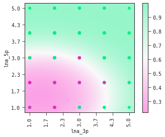
Observe how the amount of LNA modifications in the 5’ flank has a stronger effect on its toxicity than the amount of modifications in the 3’ flank.
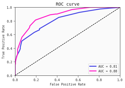
Below are the ROC curves of each region with their respective AUC scores:
best_model.plot_roc_curve(train)
best_model.plot_roc_curve(test, ax=plt.gca())