Automobile MPG

by: Chris Cave

Feyn version: 2.1+

Last updated: 24/09/2021

Here we use the QLattice to predict the miles per gallon (MPG) of cars based on other attributes such as:

• The number of cylinders,
• The horsepower,
• Its weight,
• The year it was made.

You can find this dataset and further descriptions of the features on UCI Machine Learning Repository.

import pandas as pd
import feyn
import numpy as np

from sklearn.model_selection import train_test_split

Data clean up

There are some missing values for horsepower. What we will do is just replace them with the mean value of that variable.

data = pd.read_csv("../data/auto_mpg.csv")

# Car name is a unique identifier so we remove it from training
data = data.drop("car name", axis=1)

# Obtain the mean of the horsepower
data_wo_na = data.query("horsepower != '?'").astype({"horsepower": int})
horsepower_mean = data_wo_na["horsepower"].mean()

# Replace the missing values '?' with the mean
data = data.replace(to_replace="?", value=horsepower_mean)
data = data.astype({"horsepower": int})

data.head()

	mpg	cylinders	displacement	horsepower	weight	acceleration	model year	origin
0	18.0	8	307.0	130	3504	12.0	70	1
1	15.0	8	350.0	165	3693	11.5	70	1
2	18.0	8	318.0	150	3436	11.0	70	1
3	16.0	8	304.0	150	3433	12.0	70	1
4	17.0	8	302.0	140	3449	10.5	70	1

Connect to the QLattice

Here we split the data into train and test. There are 398 samples, which is quite small. We will make the split into equal parts so we have bigger protection against overfitting.

random_state=42

train, test = train_test_split(data, test_size=0.5, random_state=random_state)

ql = feyn.connect_qlattice()
ql.reset(random_state)

Use auto_run to obtain fitted models

models = ql.auto_run(train, output_name="mpg", n_epochs=20)

Summary plot to evaluate performance

Here we evaluate the final performance of the model with useful metrics and plots.

best = models[0]
best.plot(train, test)

Training Metrics

Test

Pretty great performance with few features! We can see how simple the model is and yet still captures a lot of the signal in the data!

Plot model response

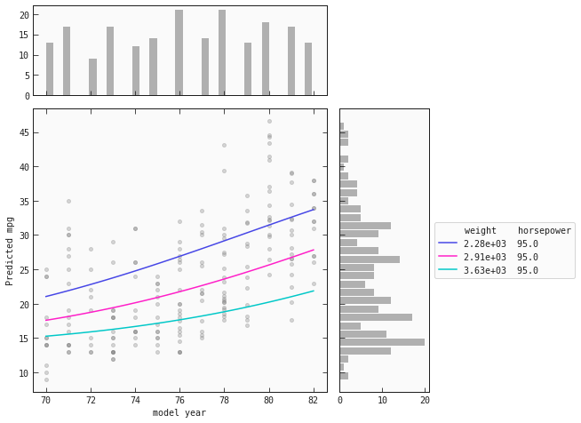
Here we will use plot_response_1d to see how the model behaves under different contraints.

best.inputs

['model year', 'weight', 'horsepower']

# This will be the input along the x-axes
x_axes = best.inputs[0]

# This will be the different colours where each colour represents the input at quartiles 25%, 50%, 75%
colours = {best.inputs[1]: train[best.inputs[1]].quantile(q=[0.25,0.5, 0.75]).values}

quantiles = train["model year"].quantile(q=[0.25,0.5, 0.75]).values

best.plot_response_1d(train, by=x_axes, input_constraints=colours)