Titanic survival
by: Meera Machado & Chris Cave
Feyn version: 2.1.+
Last updated: 23/09/2021
In this tutorial, we'll be using Feyn and the QLattice to solve a binary classification problem by exploring models that aim to predict the probability of surviving the disaster of the RMS Titanic during her maiden voyage in April of 1912.
import numpy as np
import pandas as pd

import feyn
from sklearn.model_selection import train_test_split

import matplotlib.pyplot as plt
%matplotlib inline
Importing dataset and quick check-up
The Titanic passenger dataset was acquired through the data.world and Encyclopedia Titanica websites.
df = pd.read_csv('../data/titanic.csv')
df.head()
| pclass | survived | name | sex | age | sibsp | parch | ticket | fare | cabin | embarked | boat | body | home.dest | |
|---|---|---|---|---|---|---|---|---|---|---|---|---|---|---|
| 0 | 1 | 1 | Allen, Miss. Elisabeth Walton | female | 29.0000 | 0 | 0 | 24160 | 211.3375 | B5 | S | 2 | NaN | St Louis, MO |
| 1 | 1 | 1 | Allison, Master. Hudson Trevor | male | 0.9167 | 1 | 2 | 113781 | 151.5500 | C22 C26 | S | 11 | NaN | Montreal, PQ / Chesterville, ON |
| 2 | 1 | 0 | Allison, Miss. Helen Loraine | female | 2.0000 | 1 | 2 | 113781 | 151.5500 | C22 C26 | S | NaN | NaN | Montreal, PQ / Chesterville, ON |
| 3 | 1 | 0 | Allison, Mr. Hudson Joshua Creighton | male | 30.0000 | 1 | 2 | 113781 | 151.5500 | C22 C26 | S | NaN | 135.0 | Montreal, PQ / Chesterville, ON |
| 4 | 1 | 0 | Allison, Mrs. Hudson J C (Bessie Waldo Daniels) | female | 25.0000 | 1 | 2 | 113781 | 151.5500 | C22 C26 | S | NaN | NaN | Montreal, PQ / Chesterville, ON |
Dealing with missing data
# Checking which columns have nan values:
df.columns[df.isna().any().values].to_list()
['age', 'cabin', 'boat', 'body', 'home.dest']
Among all the input features containing NaN values, age is the one of most interest.
df[df.age.isna()]
| pclass | survived | name | sex | age | sibsp | parch | ticket | fare | cabin | embarked | boat | body | home.dest | |
|---|---|---|---|---|---|---|---|---|---|---|---|---|---|---|
| 816 | 3 | 0 | Gheorgheff, Mr. Stanio | male | NaN | 0 | 0 | 349254 | 7.8958 | NaN | C | NaN | NaN | NaN |
| 940 | 3 | 0 | Kraeff, Mr. Theodor | male | NaN | 0 | 0 | 349253 | 7.8958 | NaN | C | NaN | NaN | NaN |
We take the following approach to guessing the missing ages: a random number between and , where and are, respectively, the mean age and standard deviation of all people sharing the same feature values.
age_dist = df[(df.pclass == 3) & (df.embarked == 'C') & (df.sex == 'male') &
              (df.sibsp == 0) & (df.parch == 0) & (df.survived == 0)].age.dropna()

mean_age = np.mean(age_dist)
std_age = np.std(age_dist)

np.random.seed(42)
age_guess = np.random.normal(mean_age, std_age, size=2)
# In a simple manner, we drop some features which could be irrelevant (at first look)
df_mod = df.drop(['boat', 'body', 'home.dest', 'name', 'ticket', 'cabin'], axis=1)
df_mod.loc[df[df.age.isna()].index, 'age'] = age_guess
Training session
Splitting data in train, validation and holdout sets
We wish to make a prediction on the probability of surviving the Titanic sinking, so we set survived to be our output variable.
output = 'survived'

# Train and test
train, test = train_test_split(df_mod, test_size=0.4, random_state=42, stratify=df_mod[output])

# Validation and holdout:
valid, hold = train_test_split(test, test_size=0.4, stratify=test[output], random_state=42)
Connect to QLattice
First we connect to a QLattice. Here we connect to the community QLattice
ql = feyn.connect_qlattice() # Connecting
Specify categorical variables
stypes = {}

for col in train.columns:
    if train[col].dtype == 'O':
        stypes[col] = 'c'

stypes['pclass'] = 'c' # Making sure that pclass, which is of int type, is considered a categorical variable
Sample and fit models
This occurs in the following steps:
- Sample models from the
QLattice; - Fit the models by minimizing
bic; - Update the
QLatticewith the best models' structures; - Repeat the process;
This is all captured within the auto_run function
# Resetting
ql.reset(random_seed=42)
models = ql.auto_run(train, output, kind='classification', stypes=stypes)
The model above is the one that returns the lowest bic during fitting.
best_model = models[0]
Model evaluation
best_model.plot(train, valid)
Training Metrics

Test

On the right we display a few classification metrics for train and valid ("Test").
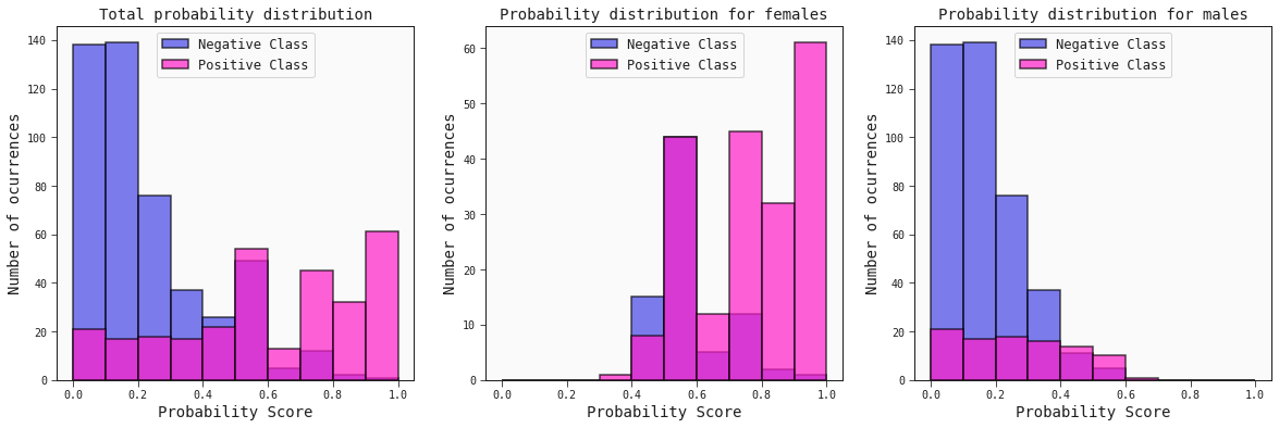
Histograms of the probability scores
The idea here consists of checking the probability distribution scores for the positive (survivors) and negative (non-survivors) classes.
fig, ax = plt.subplots(1, 3, figsize=(20, 6))
best_model.plot_probability_scores(train, title='Total probability distribution', ax=ax[0])
best_model.plot_probability_scores(train.query('sex == "female"'), title='Probability distribution for females', ax=ax[1])
best_model.plot_probability_scores(train.query('sex == "male"'), title='Probability distribution for males', ax=ax[2])
plt.show()
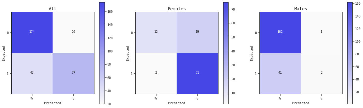
Confusion matrix
fig, ax = plt.subplots(1, 3, figsize=(20, 6))
best_model.plot_confusion_matrix(valid, ax=ax[0], title='All')
best_model.plot_confusion_matrix(valid.query('sex == "female"'), ax=ax[1], title='Females')
best_model.plot_confusion_matrix(valid.query('sex == "male"'), ax=ax[2], title='Males')
Partial plots
Below are partial dependence plots (PDP) for females and males separately:
train_f = train.query('sex == "female"').copy()
best_model.plot_response_1d(train_f, by='age', input_constraints={'pclass': [1,2,3], 'sibsp': train_f['sibsp'].median()})
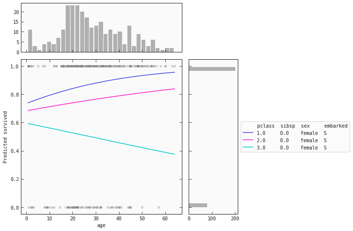
For women we see that the same behaviour is present for the and classes: as age increases, so does their chance of survival. However, the opposite happens for women in the class! As their age increases, their chance of survival decreases.
train_m = train.query('sex == "male"').copy()
best_model.plot_response_1d(train_m, by='age', input_constraints={'sex': 'male', 'pclass': [1,2,3], 'sibsp': train_m['sibsp'].median()})
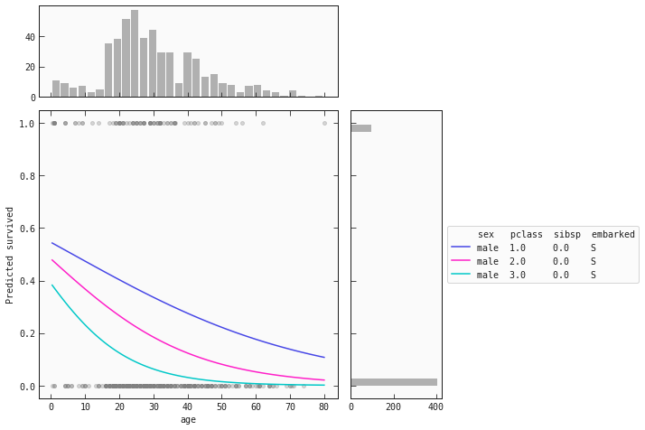
The trend for men remains the same throughout the classes: as age increases, the chance of survival decreases. However, male children have a probability score above 0.5.