Covid-19 RNA vaccine degradation data set
by: Chris Cave, Kevin Broløs and Sam Demharter
Feyn version: 2.1+
Last updated: 23/09/2021
In this tutorial we are going to go through a typical QLattice workflow. We perform an analysis on the OpenVaccine: COVID-19 mRNA Vaccine Degradation Prediction dataset.
The raw dataset consists of 2400 mRNA samples. Each mRNA consists of 107 nucleotides and various measurments were performed on the first 68 nucleotides. These measurements consisted of reactivity, degradation at pH10 with and without magnesium, and degradation at with and without magnesium.
Some of the Covid-19 vaccines are mRNA based. However due to the unstable nature of mRNA they must be refrigerated in extreme conditions. What this means is that distribution of the vaccine can be problematic.
The aim of this tutorial is to gain insights into the stability of general mRNA samples with the potential to apply it to Covid-19 vaccine candidates.
import numpy as np
import pandas as pd
import matplotlib.pyplot as plt

import feyn
from sklearn.model_selection import train_test_split

from IPython.display import display
Inspecting the raw data
Here we can see that the data we have is the sequence and the predicted structure and loop type of each base in the RNA. The feature reactivity measures the degradation at each base. The higher the reactivity the more likely the RNA is to degrade at that base.
data = pd.read_json('../data/covid_mrna.json', lines=True)
data = data.drop('index', axis=1)
data.query('SN_filter == 1', inplace=True)

length = len(data.iloc[0]['reactivity'])
first_68 = data['structure'].apply(lambda x : x[0: length])

# Remove sequences that only contain “.” i.e. unpaired bases
idx_all_dots = [i for i in first_68.index if first_68[i].count('.') == length]
data = data.drop(idx_all_dots)
data.head()
| id | sequence | structure | predicted_loop_type | signal_to_noise | SN_filter | seq_length | seq_scored | reactivity_error | deg_error_Mg_pH10 | deg_error_pH10 | deg_error_Mg_50C | deg_error_50C | reactivity | deg_Mg_pH10 | deg_pH10 | deg_Mg_50C | deg_50C | |
|---|---|---|---|---|---|---|---|---|---|---|---|---|---|---|---|---|---|---|
| 0 | id_001f94081 | GGAAAAGCUCUAAUAACAGGAGACUAGGACUACGUAUUUCUAGGUA... | .....((((((.......)))).)).((.....((..((((((...... | EEEEESSSSSSHHHHHHHSSSSBSSXSSIIIIISSIISSSSSSHHH... | 6.894 | 1 | 107 | 68 | [0.1359, 0.20700000000000002, 0.1633, 0.1452, ... | [0.26130000000000003, 0.38420000000000004, 0.1... | [0.2631, 0.28600000000000003, 0.0964, 0.1574, ... | [0.1501, 0.275, 0.0947, 0.18660000000000002, 0... | [0.2167, 0.34750000000000003, 0.188, 0.2124, 0... | [0.3297, 1.5693000000000001, 1.1227, 0.8686, 0... | [0.7556, 2.983, 0.2526, 1.3789, 0.637600000000... | [2.3375, 3.5060000000000002, 0.3008, 1.0108, 0... | [0.35810000000000003, 2.9683, 0.2589, 1.4552, ... | [0.6382, 3.4773, 0.9988, 1.3228, 0.78770000000... |
| 2 | id_006f36f57 | GGAAAGUGCUCAGAUAAGCUAAGCUCGAAUAGCAAUCGAAUAGAAU... | .....((((.((.....((((.(((.....)))..((((......)... | EEEEESSSSISSIIIIISSSSMSSSHHHHHSSSMMSSSSHHHHHHS... | 8.800 | 1 | 107 | 68 | [0.0931, 0.13290000000000002, 0.11280000000000... | [0.1365, 0.2237, 0.1812, 0.1333, 0.1148, 0.160... | [0.17020000000000002, 0.178, 0.111, 0.091, 0.0... | [0.1033, 0.1464, 0.1126, 0.09620000000000001, ... | [0.14980000000000002, 0.1761, 0.1517, 0.116700... | [0.44820000000000004, 1.4822, 1.1819, 0.743400... | [0.2504, 1.4021, 0.9804, 0.49670000000000003, ... | [2.243, 2.9361, 1.0553, 0.721, 0.6396000000000... | [0.5163, 1.6823000000000001, 1.0426, 0.7902, 0... | [0.9501000000000001, 1.7974999999999999, 1.499... |
| 5 | id_00ab2d761 | GGAAAGCGCCGCGGCGGUAGCGGCAGCGAGGAGCGCUACCAAGGCA... | .....(.(((((.(((((((((...........)))))))..(((.... | EEEEESISSSSSISSSSSSSSSHHHHHHHHHHHSSSSSSSMMSSSH... | 4.136 | 1 | 107 | 68 | [0.1942, 0.2041, 0.1626, 0.1213, 0.10590000000... | [0.2726, 0.2984, 0.21660000000000001, 0.1637, ... | [0.3393, 0.2728, 0.2005, 0.1703, 0.1495, 0.134... | [0.165, 0.20520000000000002, 0.179, 0.1333, 0.... | [0.2864, 0.24710000000000001, 0.2222, 0.1903, ... | [0.7642, 1.6641, 1.0622, 0.5008, 0.4107, 0.133... | [0.9559000000000001, 1.9442, 1.0114, 0.5105000... | [1.9554, 2.1298, 1.0403, 0.609, 0.5486, 0.386,... | [0.22460000000000002, 1.7281, 1.381, 0.6623, 0... | [0.5882000000000001, 1.1786, 0.9704, 0.6035, 0... |
| 6 | id_00abef1d7 | GGAAAACAAUUGCAUCGUUAGUACGACUCCACAGCGUAAGCUGUGG... | .........((((((((......((((((((((((....)))))))... | EEEEEEEEESSSSSSSSIIIIIISSSSSSSSSSSSHHHHSSSSSSS... | 2.485 | 1 | 107 | 68 | [0.422, 0.5478000000000001, 0.4749000000000000... | [0.4801, 0.7943, 0.42160000000000003, 0.397300... | [0.9822000000000001, 1.272, 0.6940000000000001... | [0.5827, 0.7555000000000001, 0.5949, 0.4511, 0... | [0.9306000000000001, 1.0496, 0.5844, 0.7796000... | [0.895, 2.3377, 2.2305, 2.003, 1.9006, 1.0373,... | [0.46040000000000003, 3.6695, 0.78550000000000... | [2.7711, 7.365, 1.6924000000000001, 1.43840000... | [1.073, 2.8604000000000003, 1.9936, 1.0273, 1.... | [2.0964, 3.3688000000000002, 0.6399, 2.1053, 1... |
| 7 | id_00b436dec | GGAAAUCAUCGAGGACGGGUCCGUUCAGCACGCGAAAGCGUCGUGA... | .....(((((((((((..(((((((((..((((....))))..)))... | EEEEESSSSSSSSSSSIISSSSSSSSSIISSSSHHHHSSSSIISSS... | 1.727 | 1 | 107 | 68 | [0.4843, 0.5233, 0.4554, 0.43520000000000003, ... | [0.8719, 1.0307, 0.6649, 0.34500000000000003, ... | [0.7045, 0.7775000000000001, 0.5662, 0.4561, 0... | [0.384, 0.723, 0.4766, 0.30260000000000004, 0.... | [0.7429, 0.9137000000000001, 0.480400000000000... | [1.1576, 1.5137, 1.3382, 1.5622, 1.2121, 0.295... | [1.6912, 5.2652, 2.3901, 0.45890000000000003, ... | [1.8641, 2.3767, 1.149, 1.0132, 0.9876, 0.0, 0... | [0.49060000000000004, 4.6339, 1.95860000000000... | [1.2852000000000001, 2.5460000000000003, 0.234... |
There's a column in this data set called SN_filter. This is the signal to noise filter capturing which RNA molecules that passed the evaluation criteria defined by the Stanford researchers. This means we will drop the rows with SN_filter == 0
There are some RNAs that have quite a large amount of noise which is filtered by the SN_filter.
There are also RNAs that are all "." for the first 68 bases. During analysis, we've removed these sequences, as they were hard to capture since they have no variation in predicted structure, but a lot of variation in reactivity. This could be due to it having a very complex structure that is not represented here, or the predicted loop type being incorrect, or something entirely different.
Preparing the sequences for the QLattice
Here, we prepare the sequences for the QLattice, by expanding the sequences into individual samples for each nucleobase. This means, that each sample consists of one nucleobase (base), and a predicted loop type (loop).
In order to maintain information about its position and relevance in the structure, we add some features about its surrounding neighbours. We call these motifs.
The motifs are defined by a left-side (5') and right-side (3') window of the two neighbouring bases. We then do the same, but for the loop type.
end_pos = len(data.loc[0, 'predicted_loop_type'])

RNA_idx = [j for j in data.index for i in range(0, end_pos)]
pos_idx = [i for j in data.index for i in range(0, end_pos)]

loop_exp = data['predicted_loop_type'].apply(lambda x : list(x)).agg(sum)
base_exp = data['sequence'].apply(lambda x : list(x)).agg(sum)

exp_df = pd.DataFrame({'loop' : loop_exp, 'base': base_exp, 'RNA_idx' : RNA_idx, 'pos_idx' : pos_idx})
react_len = len(data.iloc[0].reactivity)
df = exp_df[exp_df.pos_idx < react_len]
df = df[df.pos_idx >= 5]

df['reactivity'] = df.apply(lambda row: data.loc[row.RNA_idx].reactivity[row.pos_idx], axis=1)

df['sequence'] = data.loc[df.RNA_idx].set_index(df.index).sequence
df['base_left_motif'] = df.apply(lambda x: x['sequence'][:x.pos_idx][-2:], axis=1)
df['base_right_motif'] = df.apply(lambda x: x['sequence'][x.pos_idx + 1:][:2], axis=1)

df['loop_type'] = data.loc[df.RNA_idx].set_index(df.index).predicted_loop_type
df['loop_left_motif'] = df.apply(lambda x: x['loop_type'][:x.pos_idx][-2:], axis=1)
df['loop_right_motif'] = df.apply(lambda x: x['loop_type'][x.pos_idx + 1:][:2], axis=1)
Train, validation and holdout split
We split our train/validation/holdout split according to the sequence it belongs to. This is to make sure we don't contaminate our validation and holdout sets with samples from the same sequences we have trained on. We've captured the original sequences in the column RNA_idx to make this splitting easier. We have some other meta columns like this, that we'll remove prior to training.
train_idx, remain_idx = train_test_split(list(data.index),train_size = 0.5, random_state = 42)
valid_idx, holdout_idx = train_test_split(remain_idx,train_size = 0.5, random_state = 42)

train = df.query('RNA_idx == @train_idx')
valid = df.query('RNA_idx == @valid_idx')
holdout = df.query('RNA_idx == @holdout_idx')
Here is our training set. We've expanded the previous data set so we have a feature for base, predicted loop type, base_left_motif, base_right_motif, left_loop_motif and right_loop_motif
train.head()
| loop | base | RNA_idx | pos_idx | reactivity | sequence | base_left_motif | base_right_motif | loop_type | loop_left_motif | loop_right_motif | |
|---|---|---|---|---|---|---|---|---|---|---|---|
| 5 | S | A | 0 | 5 | 0.4384 | GGAAAAGCUCUAAUAACAGGAGACUAGGACUACGUAUUUCUAGGUA... | AA | GC | EEEEESSSSSSHHHHHHHSSSSBSSXSSIIIIISSIISSSSSSHHH... | EE | SS |
| 6 | S | G | 0 | 6 | 0.2560 | GGAAAAGCUCUAAUAACAGGAGACUAGGACUACGUAUUUCUAGGUA... | AA | CU | EEEEESSSSSSHHHHHHHSSSSBSSXSSIIIIISSIISSSSSSHHH... | ES | SS |
| 7 | S | C | 0 | 7 | 0.3364 | GGAAAAGCUCUAAUAACAGGAGACUAGGACUACGUAUUUCUAGGUA... | AG | UC | EEEEESSSSSSHHHHHHHSSSSBSSXSSIIIIISSIISSSSSSHHH... | SS | SS |
| 8 | S | U | 0 | 8 | 0.2168 | GGAAAAGCUCUAAUAACAGGAGACUAGGACUACGUAUUUCUAGGUA... | GC | CU | EEEEESSSSSSHHHHHHHSSSSBSSXSSIIIIISSIISSSSSSHHH... | SS | SS |
| 9 | S | C | 0 | 9 | 0.3583 | GGAAAAGCUCUAAUAACAGGAGACUAGGACUACGUAUUUCUAGGUA... | CU | UA | EEEEESSSSSSHHHHHHHSSSSBSSXSSIIIIISSIISSSSSSHHH... | SS | SH |
Approach 1: Training a QLattice to produce highly complex models
The first approach is to connect to the QLattice, and just fit a model with a large complexity.
# Connecting to the QLattice
ql = feyn.connect_qlattice()

# Seeding the QLattice for reproducible results
ql.reset(42)
# Output variable
output = 'reactivity'

# Declaring features
features = ['base', 'loop', 'base_left_motif', 'base_right_motif', 'loop_left_motif', 'loop_right_motif']

# Declaring categorical features
stypes = {}
for f in features:
    if train[f].dtype =='object':
        stypes[f] = 'c'
In order to penalize more complex graphs that don't necessarily add enough utility compared to their simpler counterparts, we use BIC as a selection criterion prior to updating the QLattice with the best models.
This avoids redundancies in your models, so that each interaction is potentially contributing something useful whenever possible.
This is a regression task, which is default for auto_run
models = ql.auto_run(train[features+[output]], output, stypes=stypes, criterion='bic')
model_base = models[0]
model_base.plot(train)
Training Metrics

We've supplied a random seed to this QLattice, but depending on version you might still be experiencing different results, so keep that in mind as you try this for yourself.
model_base.plot_signal(train)
Looking at the plot above it appears that one of them doesn't add a lot of signal to the model - notice how the base_left_motif into the next interaction of the model doesn't seem to increase the signal by much. This is more obvious when compared to the added signal from combining the other features in the model.
Let's constrain the models
The previous plots tells us is that we should try to restrict the graph a bit more to force the QLattice to choose the best features, as it won't have room to use them all.
We can achieve this constraint by setting the max complexity to 7, which would allow for the individual models to only contain maximum 4 features.
ql.reset(42)
models = ql.auto_run(train[features+[output]], output, stypes=stypes, max_complexity=7, criterion='bic')
model_constrained = models[0]
Taking a look at the train and validation sets:
print('The base model (unconstrained):')
display(model_base.plot(train, valid))
print("The constrained model (max complexity = 7):")
display(model_constrained.plot(train, valid))
The base model (unconstrained):
Training Metrics
Test

The constrained model (max complexity = 7):
Training Metrics

Test

model_constrained.plot_signal(train)
Both of these models actually appear to generalize quite well. However, it also confirms our suspicions that the left motifs are less important.
What's next?
So we seem to have a stable model with only four features.
Now it'd be interesting to see just how far down we can carve this model until it falls apart.
We'll try to get rid of the features that seem to contribute the least.
In the above plots, it would appear that the loop_right_motif contributes the least to the growth of signal in the model, so let's try to remove it
ql.reset(42)

features = ['base', 'loop', 'base_right_motif']
models = ql.auto_run(train[features+[output]], output, stypes=stypes, max_complexity=6, criterion='bic')
model_three_features = models[0]
print('The constrained model:')
display(model_constrained.plot(train, valid))
print("The three feature model:")
display(model_three_features.plot(train, valid))
The constrained model:
Training Metrics
Test
The three feature model:
Training Metrics

Test

model_three_features.plot_signal(train)
We're very close here. It did get a little worse - but if we want to tend towards simpler, more interpretble models, the three feature model is definitely what we should go for.
It also already provides so much signal, that we can expect it to explain most of the behaviour we are able to describe using these features.
That said - we might now already also see that the base doesn't supply much information, so let's try to remove it and see how dramatic of a difference that makes.
ql.reset(42)

features = ['loop', 'base_right_motif']
# Note we're reducing to max complexity of 3 for two features.
models = ql.auto_run(train[features+[output]], output, stypes=stypes, max_complexity=3, criterion='bic')
model_two_features = models[0]
print("The three feature model:")
display(model_three_features.plot(train, valid))
print("The two feature model:")
display(model_two_features.plot(train, valid))
The three feature model:
Training Metrics
Test
The two feature model:
Training Metrics

Test

We see a bit of a drop but that's also in line with our expectations.
Still, we seem to be getting closer to the essence of the model here. The loop and the base_right_motiftogether.
We could reduce further down to just the loop - but without feature interactions it's fairly obvious that the performance would reduce to just the explanative power of the loop feature.
model_two_features.plot_signal(train)
Let's look at an interesting sequence
Now we have a few models we can take a look at an intersting sequence and try to map out what kind of tradeoffs we get over different complexities.

This is one of the sequences from the validation set. Let's start plotting the predicted reactivity and compare to the actual reactivity for the simplest model and work our way up. This picture was generated by the forna server that ViennaRNA has made available here: http://rna.tbi.univie.ac.at/forna/
Defining a useful plotting function for RNA sequences
First, let's define a function to plot the sequences of the predictions versus the actuals, to help us identify the peaks and valleys of our predictions across the sequences.
def plot_RNA_seq(model, data, idx, figsize = (24,5), grid=True, title=''):

    output = model.output
    fig, ax = plt.subplots(figsize = figsize)

    sub_seq = data.query(f'RNA_idx == {idx}')

    prediction = model.predict(sub_seq)
    ax.plot(range(len(sub_seq)), sub_seq[output], label = 'actuals')
    ax.plot(range(len(sub_seq)), prediction, label = 'pred')

    x_axis1 = list(sub_seq['loop'].values)
    x_axis2 = list(sub_seq['base'].values)

    x_axis = list(zip(x_axis1, x_axis2))
    x_axis = ["_".join(x_axis[i]) for i in range(len(x_axis))]

    ax.set_xticks(range(len(sub_seq)))
    ax.set_xticklabels(x_axis)
    ax.tick_params(rotation = 90)
    ax.set_title(title+str(idx))

    ax.set_ylabel(output)
    ax.set_xlabel('sequence (loop and base)')

    ax.legend()

    if grid:
        ax.grid()

    return ax
plot_RNA_seq(model_two_features, valid, [642])
display(model_two_features)
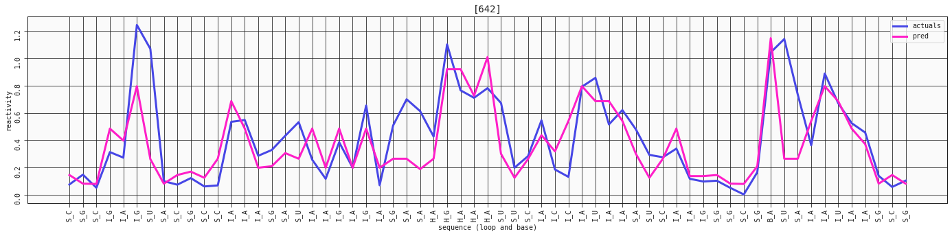
This sequence is already captured really well with the simplest, two-feature model of the loop and base_right_motif. Let's compare it with the three-feature one, that includes the base.
ax = plot_RNA_seq(model_three_features, valid, [642])
ax.annotate('Region 1', (24,0.8), bbox=dict(boxstyle="round,pad=0.3", fc='#FFE10A', lw=2))
ax.annotate('Region 2', (38,1), bbox=dict(boxstyle="round,pad=0.3", fc='#FFE10A', lw=2))
ax.annotate('Region 3', (34,0.05), bbox=dict(boxstyle="round,pad=0.3", fc='#FFE10A', lw=2))
display(model_three_features)
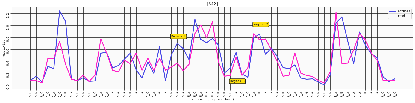
It's not the steepest difference, but we see a bit more of a defined peak at the I_A in region 2 on the plot. We also see a bit more reactivity in the S_G-S_A region 1. The I_A-I_C in region 3 is also much more closely mapped in this prediction.
In general we might see a bit more correction on the stems with the base included.
ax = plot_RNA_seq(model_constrained, valid, [642])
ax.annotate('Region 1', (24,0.8), bbox=dict(boxstyle="round,pad=0.3", fc='#FFE10A', lw=2))
ax.annotate('Region 2', (38,1), bbox=dict(boxstyle="round,pad=0.3", fc='#FFE10A', lw=2))
ax.annotate('Region 3', (34,0.05), bbox=dict(boxstyle="round,pad=0.3", fc='#FFE10A', lw=2))
display(model_constrained)
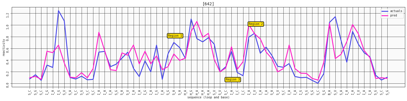
With the constrained, four feature model we're getting a little closer to some of the reactive stems in region 1, but it comes at the cost of some oversensitivity in other regions. However, looking at our three regions from before, they are now all generally better captured.
This is where it'd make sense to ask yourself what you're trying to accomplish with the model and whether to focus more on performance on specific things, or to understand the dynamics using simpler models.
ax = plot_RNA_seq(model_base, valid, [642])
ax.annotate('Region 1', (24,0.8), bbox=dict(boxstyle="round,pad=0.3", fc='#FFE10A', lw=2))
ax.annotate('Region 2', (38,1), bbox=dict(boxstyle="round,pad=0.3", fc='#FFE10A', lw=2))
ax.annotate('Region 3', (34,0.05), bbox=dict(boxstyle="round,pad=0.3", fc='#FFE10A', lw=2))
display(model_base)
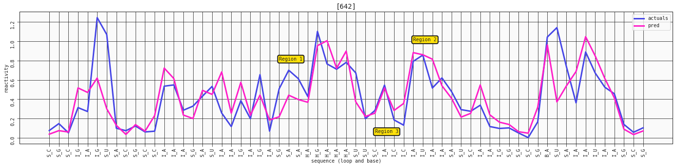
As we discovered, having these extra features doesn't really capture much more or add more to the story - it's just curve fitting at this point, trying to squeeze out every last bit of signal. You might see some better adjustments here and there, and some worse performance in other places, but nothing major like what we've seen previously.
Plotting the development of the RMSE from more complex to simpler models
print(f'RMSE model features: {len(model_base.features)}: {model_base.rmse(valid):.4f}')
print(f'RMSE model features: {len(model_constrained.features)}: {model_constrained.rmse(valid):.4f}')
print(f'RMSE model features: {len(model_three_features.features)}: {model_three_features.rmse(valid):.4f}')
print(f'RMSE model features: {len(model_two_features.features)}: {model_two_features.rmse(valid):.4f}')
RMSE model features: 5: 0.2915
RMSE model features: 4: 0.2968
RMSE model features: 3: 0.2970
RMSE model features: 2: 0.3060
Looking at this, depending on whether you want interpretability or performance, you'd be well off picking between the three or four feature graph.
Let's take a look at how they perform on the holdout set
print(f'RMSE model features: {len(model_base.features)}: {model_base.rmse(holdout):.4f}')
print(f'RMSE model features: {len(model_constrained.features)}: {model_constrained.rmse(holdout):.4f}')
print(f'RMSE model features: {len(model_three_features.features)}: {model_three_features.rmse(holdout):.4f}')
print(f'RMSE model features: {len(model_two_features.features)}: {model_two_features.rmse(holdout):.4f}')
RMSE model features: 5: 0.2912
RMSE model features: 4: 0.2957
RMSE model features: 3: 0.2971
RMSE model features: 2: 0.3070
We see a good generalization to the holdout set, and a similar story as to which complexity level to pick. This is a very good sign, and shows us that we're on the right track to a possible model on how the structure of an RNA sequence combined with the bases impacts the reactivity at each point.
Concluding remarks
In this example we showed how the QLattice can be used to produce simple models that pick out the important features describing reactivity. This gives us a better understanding of the mechanisms underlying mRNA reactivity and, because of it's simplicity, is able to generalise to unseen data sets. This is the power of the QLattice, simple and explainable models with high predictive performance on unseen data sets!