Simple linear and logistic regression

by: Miquel Triana

Feyn version: 2.1+

Fit linear and logistic regressions using feyn

The function auto_run uses, among other primitives, a gradient descent fit in order to find the best performing models. In this tutorial we will show you how to use these capabilities to find the best fit for simple models like linear and logistic regressions.

Using the query language, sample_models can be completely constrained to the functional form of our choice. To obtain a linear regression on one variable we just need to pass query_string="'x'", as all variables are transformed linearly prior to being used in the model $y = Ax + B$ For a logistic regression, passing 'classification' to the kind parameter will wrap the output with a sigmoid function $\frac{1}{1+e^{-y}}$ The resulting models will be then fit all at once using fit_models, that will return them ordered by training loss.

import numpy as np
import pandas as pd
import matplotlib.pyplot as plt
from sympy import simplify

import feyn

np.random.seed(42)

ql = feyn.connect_qlattice()
ql.reset(42)

Linear models

Let's create first a synthetic dataset to work

# parameters
a = 2
b = 1

beta_0 = -0.5
beta_1 = 4

# parameters of distribution
n_samples = 10000
spread = 0.2

# get samples for the independent variable X
x = np.sort(np.random.rand(n_samples))

# get y by evaluating linear expression + random gaussian noise
y = a*x + b + np.random.normal(scale=spread, size=n_samples)
# get y_binary by sampling binomial distribution with probabilities following sigmoid(x)
y_binary = list(map(lambda x: np.random.binomial(1, x, size=1)[0], 1/(1+np.exp(-(beta_1*x + beta_0)))))

data = pd.DataFrame({'x': x, 'y':y, 'y_binary':y_binary})

Linear regression

We sample thousands of models with random initial weights, fit all them at once, and select the one with the smallest loss

models_regression = ql.sample_models(["x"], output_name="y", kind="regression", query_string="'x'")
models_regression = feyn.fit_models(models_regression, data)

len(models_regression)

2400

Models can be easily inspected with the sympify method

models_regression[0].sympify()

$\displaystyle 1.8951 x + 0.952343$

We can call the fit_models function repeatedly to refine the fit of the parameters. With the method .loss_value you can access the train loss to evaluate its progress

regression_losses = []
epochs = 20
for i in range(epochs):
    models_regression = feyn.fit_models(models_regression, data)
    regression_losses.append(models_regression[0].loss_value)

plt.plot(range(epochs), regression_losses);
plt.xlabel("epochs");
plt.ylabel("RMSE loss");

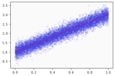
Let's inspect the final model weights, and the fitted line together with the training data

models_regression[0].sympify()

$\displaystyle 2.01907 x + 0.993852$

plt.scatter(x, y, alpha=0.1)
plt.plot(x, models_regression[0].predict(data), color="red", linewidth=1);

Logistic regression

Following the same steps as before, we can now fit a logistic regression

models_classification = ql.sample_models(["x"], output_name="y_binary", kind="classification", query_string="'x'")
models_classification = feyn.fit_models(models_classification, data)

models_classification[0].sympify()

$\displaystyle \operatorname{logreg}{\left(4.07988 x - 0.587351 \right)}$

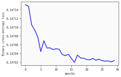
classification_losses = []
epochs = 30
for i in range(epochs):
    models_classification = feyn.fit_models(models_classification, data)
    classification_losses.append(models_classification[0].loss_value)
    
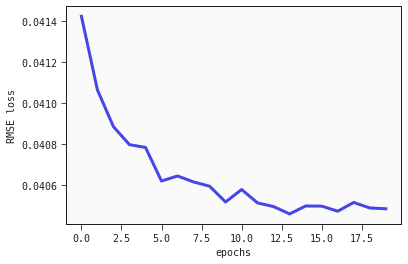
plt.plot(range(epochs), classification_losses);
plt.xlabel("epochs");
plt.ylabel("Binary cross-entropy loss");

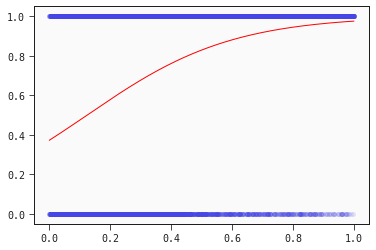
models_classification[0].sympify()

$\displaystyle \operatorname{logreg}{\left(4.19671 x - 0.519818 \right)}$

plt.scatter(x, y_binary, alpha=0.1)
plt.plot(x, models_classification[0].predict(data), color="red", linewidth=1);

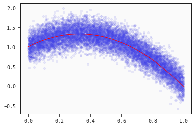
Quadratic models

But what if the data we have is clearly non-linear? We can fit a more complex funtion

# parameters of distribution
a_1 = 2
a_2 = -3
b = 1

n_samples = 10000
spread = 0.2


x = np.sort(np.random.rand(n_samples))

y = a_1*x + a_2*(x**2)+ b + np.random.normal(scale=spread, size=n_samples)

data = pd.DataFrame({'x': x, 'y':y})

Regression

models_regression = ql.sample_models(["x"], output_name="y", kind="regression", query_string="'x'+squared('x')")
models_regression = feyn.fit_models(models_regression, data)

simplify(models_regression[0].sympify())

$\displaystyle - 2.9738 x^{2} + 1.96955 x + 0.983796$

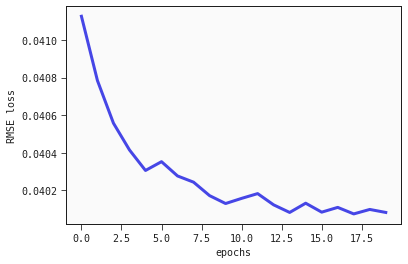
regression_losses = []
epochs = 20
for i in range(epochs):
    models_regression = feyn.fit_models(models_regression, data)
    regression_losses.append(models_regression[0].loss_value)
    
plt.plot(range(epochs), regression_losses);
plt.xlabel("epochs");
plt.ylabel("RMSE loss");

simplify(models_regression[0].sympify())

$\displaystyle - 3.02001 x^{2} + 1.98678 x + 1.00808$

plt.scatter(x, y, alpha=0.1)
plt.plot(x, models_regression[0].predict(data), color="red", linewidth=1);