Preventing the Honeybee Apocalypse (QSAR)
by: Niels Johan Christensen and Samuel Demharter
Feyn version: 2.0
Honey bees are at risk!
Many insectides are based on similar chemical scaffolds as nerve agents. Exposure to these agents leads to lethal interruption of nerve transmission by inhibition of the enzyme (acetylcholinesterase) that degrades the neurotransmitter acetylcholine.
Can we use the QLattice to make interpretable and generalisable Quantitative Structure Activity Relationship (QSAR) predictions?
I.e. in this case, can we find the combination of chemical descriptors that best predict honey bee toxicity? This model would be helpful for chemists who want to develop honey-bee-friendly pesticides.
- The target variable for this regression exercise is -log(LD50). This is a measure of toxicity of the compounds.
- The dataset we'll be looking at was published (find the model here) and included 16 chemical descriptors. Can we improve on the published model? Note, the published prediction is an ensemble average of models and thus is not very interpretable.
Reference: Dulin, F.; Halm-Lemeille, M.-P.; Lozano, S.; Lepailleur, A.; Sopkova-de Oliveira Santos, J.; Rault, S.; Bureau, R. Interpretation of honeybees contact toxicity associated to acetylcholinesterase inhibitors. Ecotoxicol. Environ. Saf. 2012, 79, 13–21. http://dx.doi.org/10.1016/j.ecoenv.2012.01.007
Let's import some libraries
import pandas as pd
import feyn
from sklearn.model_selection import train_test_split
import warnings
warnings.filterwarnings('ignore')
# Read the data
# Note, the column names are abbreviated for convenience.
df = pd.read_csv("../data/honeybee.csv", index_col=0)
df.head()
| Meaninformationindex1 | PresenceabsenceofSPa2 | PresenceabsenceofCCa3 | Lowesteigenvalue3ofB4 | RCXXRCXXCX5 | ComplementaryInforma6 | Dipolemomentcomponen7 | Gearyautocorrelation8 | Gearyautocorrelation9 | GhoseViswanadhanWend10 | Energyofthelowestuno11 | Moranautocorrelation12 | Shadowindexcomponent13 | Shadowindexcomponent14 | StructuralInformatio15 | Estatetopologicalpar16 | 48hHoneybeetoxicitya17 | |
|---|---|---|---|---|---|---|---|---|---|---|---|---|---|---|---|---|---|
| Compound Id | |||||||||||||||||
| S1 | 2.023 | 1 | 1 | 1.317 | 1 | 0.713 | -2.54264 | 1.103 | 0.000 | 0 | -0.10516 | 0.213 | 0.66986 | 0.63133 | 0.835 | 30.447 | 2.188 |
| S2 | 1.744 | 0 | 1 | 1.693 | 2 | 0.890 | -1.60728 | 1.025 | 0.997 | 0 | -0.07309 | -0.069 | 0.66613 | 0.71244 | 0.843 | 79.169 | 2.773 |
| S3 | 1.741 | 0 | 1 | 1.293 | 0 | 1.039 | 0.19352 | 1.195 | 1.286 | 0 | -0.07899 | -0.226 | 0.54579 | 0.62523 | 0.779 | 27.796 | 2.830 |
| S4 | 1.533 | 0 | 1 | 1.544 | 0 | 1.292 | -1.12375 | 1.045 | 1.944 | 0 | -0.02942 | -0.264 | 0.74537 | 0.79094 | 0.739 | 21.392 | 3.239 |
| S5 | 2.099 | 1 | 1 | 1.584 | 1 | 0.985 | -1.33811 | 0.451 | 0.720 | 1 | -0.13295 | 0.583 | 0.54227 | 0.66500 | 0.803 | 38.281 | 2.881 |
Split the data into train and test
We will use the same train/test split as in the published QSAR model
test = df.loc[['S2','S7','S25','S41','S42','S44']]
train = df.drop(index=['S2','S7','S25','S41','S42','S44'])
target = df.columns[-1]
Strategy 1: Create a linear QSAR model
Typically, QSAR models are linear. Only recently has the exploration of non-linear QSAR modelling gained traction.
Luckily we can do both with the QLattice. Let's start building a linear model and then continue with non-linear models.
To this end we:
- only allow "add" (linear) functions
- run 20 fitting loops or "epochs"
- use the bic criterion (bayesian information criterion) to keep things simple
Initialize a Community QLattice
ql = feyn.connect_qlattice()
ql.reset(random_seed=42)
Run the QLattice over 20 epochs
models = ql.auto_run(train[train.columns], target, n_epochs=20, criterion='bic',function_names = ["add"] )
Evaluate the performance on the training and test data
models[0].plot(train, test)
# Regression plot for the training set
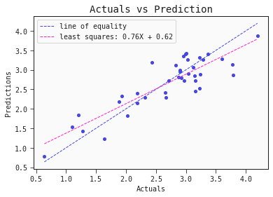
models[0].plot_regression(train)
# Regression plot for the test set
models[0].plot_regression(test)
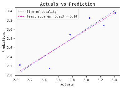
Nice! The performance of this single linear model is comparable to the performance of the ensembl model presented in the literature.
Strategy 2: Create a simple and non-linear QSAR model
Now let's do something non linear.
- We'll start out with just 3 epochs of symbolic regression while also keeping the graph complexity low (max_complexity = 3).
- We'll run the
QLatticewith the full function repertoire (in addition to "add" there are currently 9 other functions. See them listed under "interactions" here).
ql.reset(random_seed=42)
models = ql.auto_run(train[train.columns], target, max_complexity = 3, n_epochs=3)
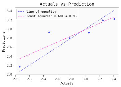
The QLattice arrives at two-descriptor only model. The test metrics look really good:
models[0].plot(train, test)
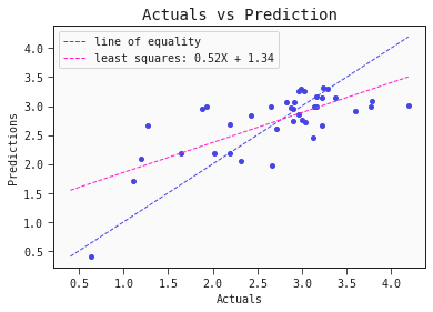
We got a decent simple model that can easily be interpreted. Two features interacting in an elegant non-linear relationship.
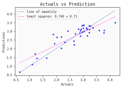
How do our predictions compare to the actual toxicity?
models[0].plot_regression(train)
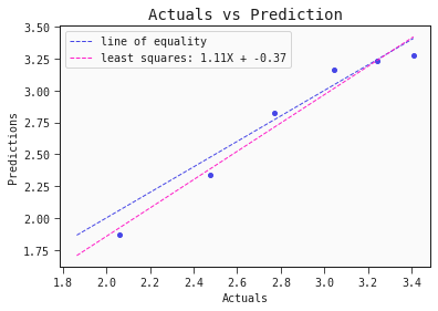
models[0].plot_regression(test)
This simple QSAR model is based on only two descriptors, namely:
- Presence/absence of S–P at topological distance 1: This descriptor encodes the presence (=1) or absence (=0) of a sulfur atom directly bound to phosphorus
- Geary autocorrelation of lag 6 weighted by Sanderson electronegativity: This particular descriptor "sums the products of atom weights of the terminal atoms of all the paths of the path length = 6 (the lag) weighted by electronegativity
- A summary of this and other autocorrelaton descriptors is found here (http://www.vcclab.org/lab/indexhlp/2dautoc.html)
Interpret the simple non-linear model
The plot_partial2d plot is useful for elucidating the interplay between molecular descriptors.
models[0].plot_partial2d(train)
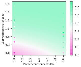
It is clear from the partial2d plots below that
- (i) increasing values of Gearyautocolation9 is associated with increased toxicity
- (ii) that the presence of a sulfur atom directly attached to phosphorous amplifies this toxicity.
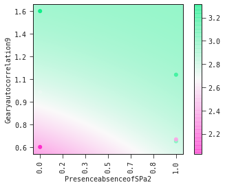
models[0].plot_partial2d(test)
Show the model as a mathematical expression
sympy_model = models[0].sympify(signif=3)
sympy_model.as_expr()
This is the model. Nothing is hidden away. You could copy and paste this formula into a excel worksheet and work with it. That's one of the benefits of symbolic regression.
Strategy 3: Full-on QLattice modelling
Can we further improve the predictive performance of our model? Let's set the QLattice loose and see what happens.
- Run the
QLatticefor 10 epochs using the bic criterion (see here for details) to keep things simple. - Keep default model complexity (max 10 edges)
ql.reset(random_seed=42)
models = ql.auto_run(train[train.columns], target, n_epochs=10, criterion='bic')
models[0].plot(train,test)
Nice R2! This model outperforms the ensemble predictions in the literature.
models[0].plot_regression(train)
models[0].plot_regression(test)
The model captures the actual toxicity surprisingly well. Note, to fully validate this model we would want to test it on another set of compounds. Also, even though the model itself is explainable, the features it includes (autocorrelation, complementary information) are hardly intuitive. More work has to be done to come up with meaningful interpretable features that also hold predictive power.
Conclusion
In this tutorial we have built linear and non-linear models using the QLattice on a typical QSAR dataset.
The smart feature selection coupled with the simplicity of the models enables researchers to rapidly explore potential mechanisms underlying the data.
This example was based on a relatively small dataset (where simple models excel). But the QLattice can readily be applied to large and wide datasets. We're looking into it ;)