Rewriting models with correlated inputs
by: Meera Machado
Feyn version: 2.1.1+
Last updated: 13/10/2021
In this tutorial we use the query language to generate models where an input variable is substituted by another variable correlated to it.
import numpy as np
import pandas as pd
import matplotlib.pyplot as plt

import feyn
from sklearn.model_selection import train_test_split
from sklearn.datasets import load_breast_cancer
Dataset and motivation
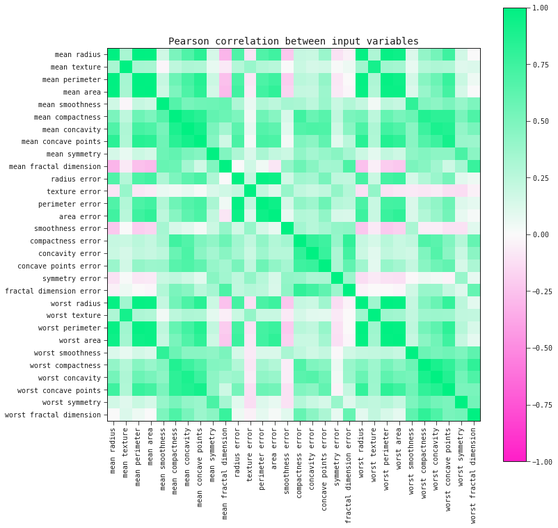
When we consider the array of data gathered for understanding diseases and diagnosing them, it is not surprising that we would find that some input variables are correlated to each other. After all, when it comes to the studying of a living being, we would expect many of its internal processes to be interconnected.
The QLattice often outputs models that do not contain all the input variables in a dataset. Therefore, it is likely that two correlated variables will not show up together in the same model and one might be chosen over the other. Then we can raise the question: can we substitute one of the input variables (in a model) by another correlated to it?
The Winsconsin Breast Cancer dataset is ideal to tackle this input-swapping workflow due to some of its variables being highly correlated.
data_dict = load_breast_cancer()
data = pd.DataFrame(data=data_dict['data'], columns=data_dict['feature_names'])
data['target'] = data_dict['target']
corr_matrix = data.drop('target', axis=1).corr()

fig, ax = plt.subplots(figsize=(12, 12))
im = ax.imshow(corr_matrix.values, cmap="feyn-diverging", vmin=-1, vmax=1)
plt.colorbar(im, ax=ax)

ax.set_xticks(np.arange(len(corr_matrix.columns)))
ax.set_yticks(np.arange(len(corr_matrix.index)))

ax.set_xticklabels(corr_matrix.columns, rotation=90)
ax.set_yticklabels(corr_matrix.index)

plt.title('Pearson correlation between input variables')
plt.show()
Training session
Train-validation-holdout split
rseed = 6095
train, test = train_test_split(data, test_size=0.4, stratify=data['target'], random_state=rseed)
validation, holdout = train_test_split(test, test_size=0.5, stratify=test['target'], random_state=rseed)
Running QLattice
We run the QLattice as usual to extract a nice model where we will perform the input-swapping:
ql = feyn.connect_qlattice()
ql.reset(rseed)
models = ql.auto_run(train, 'target', kind='classification', n_epochs=20)
best_model = models[0]
Swapping inputs
Let's select the model input whose Pearson correlation's absolute value to another input variable is the highest:
# Correlations for the inputs of interest (train set)
corr_matrix_inputs = train.drop('target', axis=1).corr()
corr_matrix_inputs = corr_matrix_inputs.loc[:, best_model.inputs]

# Same pairs are not interesting
for inp in best_model.inputs:
    corr_matrix_inputs.loc[inp, inp] = np.nan
Extracting the pair with highest Pearson correlation:
# Highest correlated pair for each input
highest_pairs = np.abs(corr_matrix_inputs).idxmax(axis=0)

# Getting the values themselves
highest_corr_values = []

for inp in best_model.inputs:
    candidate = highest_pairs.loc[inp]
    value = corr_matrix_inputs.loc[candidate, inp]
    highest_corr_values.append([inp, candidate, value])

highest_corr_values = pd.DataFrame(highest_corr_values, columns=['input', 'candidate', 'corr'])

# Extract the pair with highest Pearson correlation value
max_pair = highest_corr_values.sort_values('corr', ascending=False).iloc[0]
Next we will substitute the input above by its candidate in our best_model.
From Model to query_string
An straightforward way to generate the same Model architecture as best_model while swapping one of its inputs with another variable is via the query language.
# First we go from the `Model` to its `query_string` representation:
bm_query_str = best_model.to_query_string()

# Then we swap the original input in `best_model` with the chosen candidate:
bm_query_str = bm_query_str.replace(max_pair['input'], max_pair['candidate'])
Training again
Lastly, we generate and train new models with the substituted input by passing the query_string above:
models_subst = ql.auto_run(train, 'target', kind='classification', query_string=bm_query_str, n_epochs=2)
best_subst = models_subst[0]
Comparing the models
Was there an improvement over the original best_model?
from IPython.display import display
display(best_model.plot(train, validation))
display(best_subst.plot(train, validation))
Training Metrics

Test

Training Metrics

Test
