Complexity-Loss Trade-Off
by: Emil Larsen
Feyn version: 2.1.0+
In this tutorial we will use the QLattice to compute an approximation of the Pareto front of solutions with respect to model complexity and loss. The Pareto front will give us an impression of the trade-off between model complexity and loss for models generated by the QLattice for a given data set.
Pareto Front Definition
Initially we recall the formal definition of a Pareto front:
Let , be solutions, the fitness function (higher is better) and the model complexity (lower is better). Then (Neumann, 2012):
- weakly dominates (denoted by ) if and only if
- dominates (denoted by ) if and only if
- and are incomparable if neither nor
A solution is called Pareto optimal if it is not dominated by any other solution in the search space. The set of Pareto optimal solutions is called the Pareto optimal set and the set of corresponding objective vectors is called the Pareto front.
Imports
import feyn
import pmlb
import pandas as pd
import numpy as np
import matplotlib.pyplot as plt
from sklearn.model_selection import train_test_split
from collections import namedtuple
Load Data Set
We will use the data set 207_autoPrise from the Penn Machine Learning Benchmarks (Romano et al. 2012) data set suite (link to Pandas profile report: https://epistasislab.github.io/pmlb/profile/207_autoPrice.html). The data set has 159 observations and 15 features; one of which is categorical. There are no missing values, so we can readily use the data set. We first split the data set in a train-test split and define the stypes:
data = pmlb.fetch_data(dataset_name="207_autoPrice")
train, test = train_test_split(data, test_size=0.33, random_state=42)
stypes = {'symboling': 'c'}
Run the QLattice
We start by running the QLattice 20 epochs for complexity levels ranging from 1 through 15. For each complexity level we filter out models with a different complexity level before making updates to the QLattice. After each run we collect the best performing models in a list, which we will compute the Pareto front based on. We use loss as criterion in every run.
By setting up the training loop this way with restrictions on the model complexity the aim is to get accurate models for every complexity level.
Had we run the QLattice once with no explicit restriction on the model complexity and used BIC as criterion the search would yield the model that should generalise the best to out-of-sample data, which would be sufficient in a normal use case.
The training loop is given below. We use the feyn primitives and a custom filter function set up in a two layer loop as described above.
ql = feyn.connect_qlattice()

models_all_complexity_levels = []
for complexity_level in range(1, 16):
    models = []
    ql.reset(random_seed=complexity_level)
    for epoch in range(20):
        models += ql.sample_models(train, output_name='target', kind="regression", stypes=stypes)
        models = list(filter(lambda m: m.edge_count == complexity_level, models))
        models = feyn.fit_models(models, train, criterion=None)
        models = feyn.prune_models(models)
        ql.update(models)
    models_all_complexity_levels.extend(models)
Compute Pareto Front
We can now compute the Pareto front based on the definition stated earlier. For simplicity and readability we implement this naively here directly based on the definition. You can definitely optimise this, but will not be the focus of this tutorial.
ParetoPoint = namedtuple('ParetoPoint', ['loss', 'complexity'])

def weakly_dominates(p1, p2):
        return p1.loss <= p2.loss and p1.complexity <= p2.complexity

def strictly_dominates(p1, p2):
    return weakly_dominates(p1, p2) and (p1.loss < p2.loss or p1.complexity < p2.complexity)

def compute_pareto_front(models):
    frontier = set()
    model_losses = [feyn.metrics.rmse(train['target'], m.predict(train)) for m in models]
    model_edge_counts = [m.edge_count for m in models]
    frontier = [ParetoPoint(loss, edges) for loss, edges in zip(model_losses, model_edge_counts)]
    frontier = {p for p in frontier if not any([strictly_dominates(p_prime, p) for p_prime in frontier])}

    return sorted(list(frontier), key=lambda p: p.loss)
pareto_front = compute_pareto_front(models_all_complexity_levels)
Pareto Front Plot
Finally, we plot the approximation of the Pareto front approximation as a scatter plot with steps between points.
x, y = list(zip(*pareto_front))

plt.figure()
plt.step(x, y)
plt.scatter(x, y, marker='D')
plt.yticks(ticks=range(min(y), max(y)+1), labels=range(min(y), max(y)+1))
plt.xlabel("RMSE")
plt.ylabel("Edges")
plt.show()
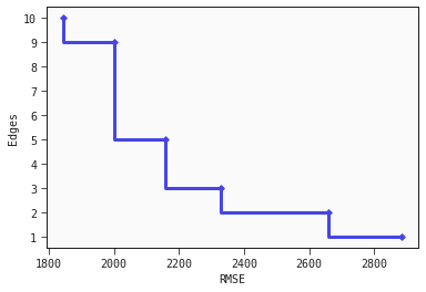
Looking at the plot we see among other things that we would have to accept a considerable increase in loss if we want a model with only one edge instead of three edges compared to the loss increase from choosing a model with five edges instead of nine edges.
Next steps from here could be to select a trade-off between model loss and complexity that we like, retrain a model with that complexity level on the whole training data and evaluate the performance on the held-out test set.
References
- Frank Neumann. Computational complexity analysis of multi-objective genetic programming. In: Proceedings of the 14th Annual Conference on Genetic and Evolutionary Computation. 2012, pp. 799-806.
- Joseph D. Romano, Trang T. Le, William La Cava, John T. Gregg, Daniel J. Goldberg, Natasha L. Ray, Praneel Chakraborty, Daniel Himmelstein, Weixuan Fu, and Jason H. Moore. PMLB v1.0: an open source dataset collection for benchmarking machine learning methods. 2021. arXiv: 2012.00058.