Plot response 1D

by: Kevin Broløs and Chris Cave
(Feyn version 3.0 or newer)

---

A Model is a mathematical function from the inputs to the output. If there are more than two inputs in a Model then it is difficult to visualise how the inputs affect the output.

One way to overcome this is to simplifiy the Model by fixing all the inputs except for one. This simplified Model now has one input and one output. This can be visualised by plotting the single input against the output. plot_response_1d enables you to choose and plot simplified models.

Example

import feyn

from sklearn.datasets import load_diabetes
import pandas as pd

from feyn.tools import split

# Load diabetes dataset into a pandas dataframe
dataset = load_diabetes()
df_diabetes = pd.DataFrame(dataset.data, columns=dataset.feature_names)
df_diabetes['response'] = dataset.target

# Train/test split
train, test = split(df_diabetes, ratio=[0.6, 0.4], random_state=42)

# Instantiate a QLattice
ql = feyn.QLattice(random_seed=42)

models = ql.auto_run(
    data=train,
    output_name='response'
)
# Select the best Model
best = models[0]
best

Plotting the model response

Static Mode

Interactive Mode

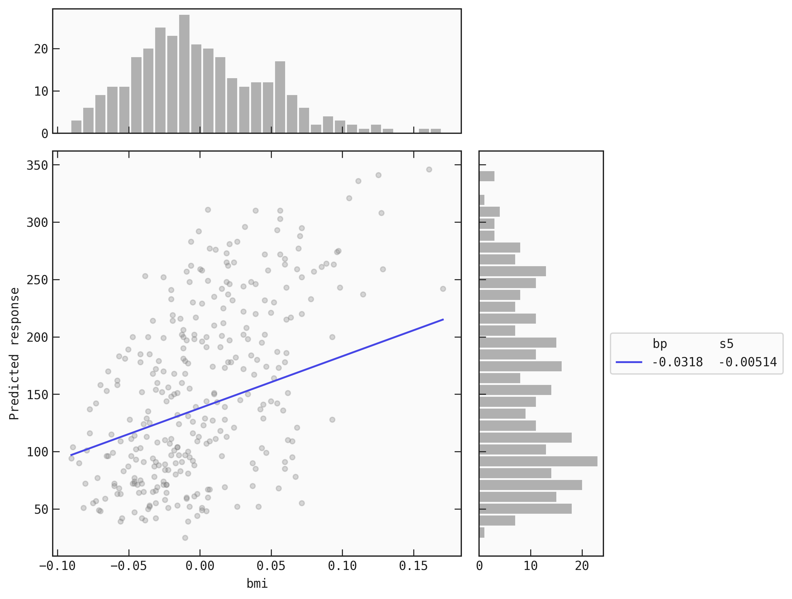
# Plot simplified model with only 'bp' manually fixed
best.plot_response_1d(
    data = train,
    by = 'bmi',
    input_constraints = {'bp': train.bmi.quantile(0.25)}
)

# Plot simplified model with only 'bp' manually fixed
best.interactive_response_1d(
    data = train,
    input_constraints = {'bp': train.bmi.quantile(0.25)}
)

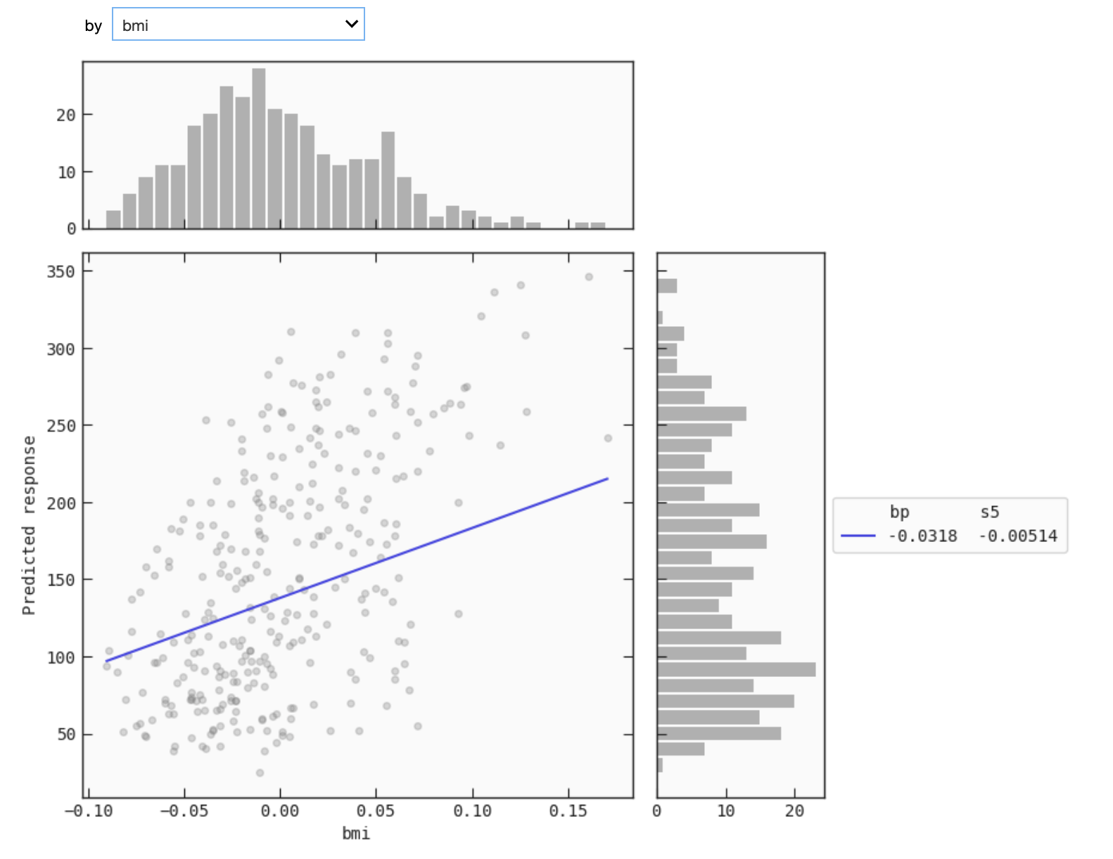
This mode that is available only for IPython kernels allows you to select the variable you want to evaluate the response as a function of. This requires installing ipywidgets and enabling the extension in jupyter notebook:

$ jupyter nbextension enable --py widgetsnbextension

or in jupyter lab:

$ jupyter labextension install @jupyter-widgets/jupyterlab-manager

---

The continuous line is the plot of the simplified function. The scatter points are the values (data[by], data[output]). The histogram on the top is of data[by] and the histogram to the side is of data[output].

Saving the plot

You can save the plot using the filename parameter. The plot is saved in the current working directory unless another path specifed.

best.plot_response_1d(
    data = train,
    by = 'bmi',
    input_constraints = {'bp': train.bmi.quantile(0.25)},
    filename="feyn-plot"
)

If the extension is not specified then it is saved as a png file.

---

Parameters of plot_response_1d

data

A pd.DataFrame of your data. This parameter is passed to determine the range of the non-fixed input to plot. All input names of the Model should be the name of columns in the data.

The data is also used to plot the scatter points. This is useful to visualise if the Model has had enough data points to say with confidence the output value of particular inputs.

by

The input name that is not fixed and is the single input of the simplified Model.

input_constraints

A dictionary where the keys are the names of all fixed inputs and the values are what to fix the Model at. If None and there are fewer than three inputs then 25%, 50% and 75% quartiles of each fixed input is passed. If there are more than three inputs then only the median is passed for each fixed input. Default is None.

Location in Feyn

This function can also be found in feyn.plots module.

from feyn.plots import plot_model_response_1d

plot_model_response_1d(best, train, 'bmi')