Plot response 2D

by: Meera Machado
(Feyn version 3.0 or newer)

The plot_response_2d function enables the visualisation of the Model response as we vary two of its features. For a Model with more then two inputs, we should assign fixed values for the remaining input features. The Model response will then be a function of the non-fixed (variable) features.

Below is an example:

import feyn
import pandas as pd
from sklearn.datasets import load_breast_cancer
from sklearn.model_selection import train_test_split


# Load into a pandas dataframe
breast_cancer = load_breast_cancer(as_frame=True)
data = breast_cancer.frame

# Train/test split
train, test = train_test_split(data, test_size=0.4, stratify=data['target'], random_state=666)

# Instantiate a QLattice
ql = feyn.QLattice(random_seed=666)

# Sample and fit models
models = ql.auto_run(
    data=train,
    output_name='target',
    kind='classification',
    max_complexity=7
)

best = models[0]

# Fixing two input features
best.plot_response_2d(
    data=train,
    fixed={
        'mean concave points': train['mean concave points'].mean(),
        'worst texture': train['worst texture'].median()
    }
)

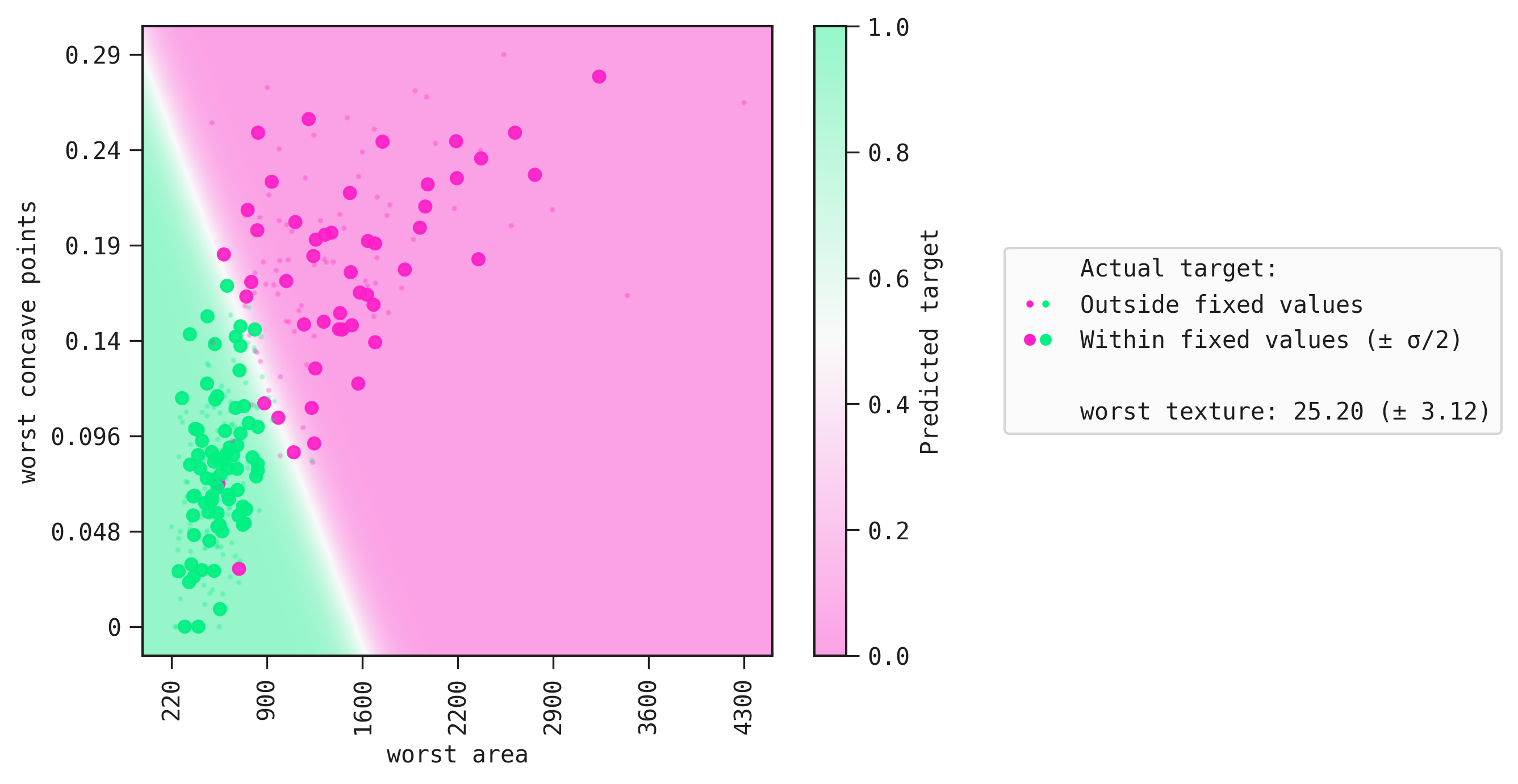
By fixing the values of mean concave points and worst texture, the function plot_response_2d plots the Model response with varying worst smoothness and worst radius. We can clearly see the boundary that separates the positive class from the negative class. Lastly, large markers are the samples whose values correspond to those in fixed.

data

The data to be analysed. It should be a pandas.DataFrame.

fixed

A dictionary where the keys are the names of the input features to be fixed and the values are the numbers/categories the features should be fixed to. The value corresponding to each key should be a scalar.

Saving the plot

You can save the plot using the filename parameter. The plot is saved in the current working directory unless another path specifed.

best.plot_response_2d(
    data=train,
    fixed={
        'mean concave points': train['mean concave points'].mean(),
        'worst texture': train['worst texture'].median(),
    },
    filename="feyn-plot"
)

If the extension is not specified then it is saved as a png file.

Location in Feyn

This function can also be found in the feyn.plots module.

from feyn.plots import plot_model_response_2d

plot_model_response_2d(
    model=best,
    data=train,
    fixed={
        'mean concave points': train['mean concave points'].mean(),
        'worst texture': train['worst texture'].median()
    }
)